5.9 Solution Validity

The reduced row-echelon form of a matrix representing a system of linear equations can be easily inspected to determine if the solution is valid or complete. But note a completely reduced form cannot always be obtained.

Test 1. A system of n equations in n unknowns has a single solution if the unaugmented portion of the reduced row-echelon matrix is an identity matrix.

Test 2. If a row in the unaugmented matrix is all zeroes and the corresponding constant is not zero, the solution is inconsistent.

Test 3. If trailing zero rows are removed and the result has fewer rows than variables, there is an infinite solution that can be expressed by allowing the missing variables to range. This is also the case when a less-than-square unaugmented matrix has insufficient information to be reduced all the way to a partial identity.

Test 2 can be seen to be inconsistent because it results in an expression like 0=2 which is patently false.

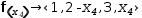
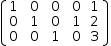
Test 3 is harder to interpret. Each missing row represents a missing linear equation in the solution set. For example, a three-row solution to a system of equations involving four variables has no solution for the last variable. This usually means that at least one row contains a value in the fourth column that violates the definition of reduced-echelon form. If this is the case, it also means that the equation form of that row will contain at least two terms.

For example,

converted to linear form is (x_1=1, x_2+x_4=2, x_3=3)ℓ. Minor manipulation of the second equation gives the solution (x_1=1, x_2=2-x_4, x_3=3)ℓ. There are two problems with this. One is that x_4 is not defined. The second is that the tuple should contain four elements, not three.

The resolution to these difficulties lies in part in recognizing that a “unique solution” is a point, in 4-space in this case. Another part lies in recognizing that x_4 is allowed an infinite number of values. This leads us to realize that the first three elements of a solution are functions of the fourth, and this is an idea naturally expressed by a function of x_4 whose result is a 4-vector. That is, for the example above, fʋ(x_4)→(1, 2-x_4, 3, x_4)ʋ. Binding the parameter x_4 to any real value and evaluating the function provides a single point. Allowing the parameter to range provides points on a line.